Clustering with the squared-loss mutual information

The squared-loss mutual information (SMI) Is a variant of mutual information proposed in [1]

In this variant, the Pearson divergence is considered as replacement for the KL divergence. The resulting cost function can be used with any clustering architecture.

We show in this example how to combine this loss, gemclus.gemini.ChiSquareGEMINI with a kernel logistic regression.

[1]

Sugiyama, M., Yamada, M., Kimura, M., & Hachiya, H. (2011). On information-maximization clustering: Tuning parameter selection and analytic solution. ICML 2011.

/home/circleci/.local/lib/python3.10/site-packages/sklearn/base.py:474: FutureWarning: `BaseEstimator._validate_data` is deprecated in 1.6 and will be removed in 1.7. Use `sklearn.utils.validation.validate_data` instead. This function becomes public and is part of the scikit-learn developer API.
  warnings.warn(
1.0

from gemclus.linear import LinearModel
from gemclus.gemini import ChiSquareGEMINI
from sklearn import datasets, metrics
from sklearn.metrics import pairwise
from matplotlib import pyplot as plt
import numpy as np

# Create the dataset
X, y = datasets.make_circles(n_samples=200, factor=0.1, noise=0.05, random_state=0)
# Center data
X = (X-X.mean(0))/X.std(0)

# Compute the kernel
kernel = pairwise.pairwise_kernels(X, metric="rbf")

# Create the linear model
model = LinearModel(n_clusters=2,  gemini=ChiSquareGEMINI(), random_state=0)

model.fit(kernel) # Linear regression on kernel = kernel model

y_pred = model.predict(kernel)
print(metrics.adjusted_rand_score(y, y_pred))

# we can also use generalisation to visualise the decision boundary

x_vals = np.linspace(-3, 3, num=50)
y_vals = np.linspace(-3, 3, num=50)
xx, yy = np.meshgrid(x_vals, y_vals)
grid_inputs = np.c_[xx.ravel(), yy.ravel()]
kernelised_grid_inputs = pairwise.pairwise_kernels(grid_inputs, X, metric="rbf")
zz = model.predict(kernelised_grid_inputs).reshape((50, 50))

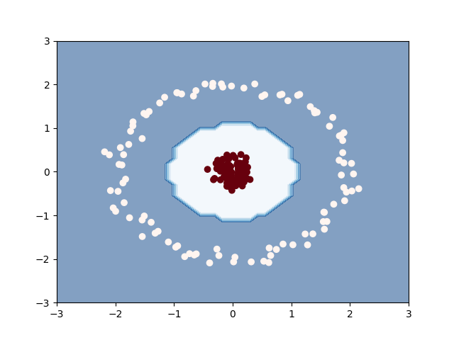
# Plot decision boundary with predictions on top
plt.contourf(xx, yy, zz, alpha=0.5, cmap="Blues")
plt.scatter(X[:, 0], X[:, 1], c=y_pred, cmap="Reds_r")
plt.show()