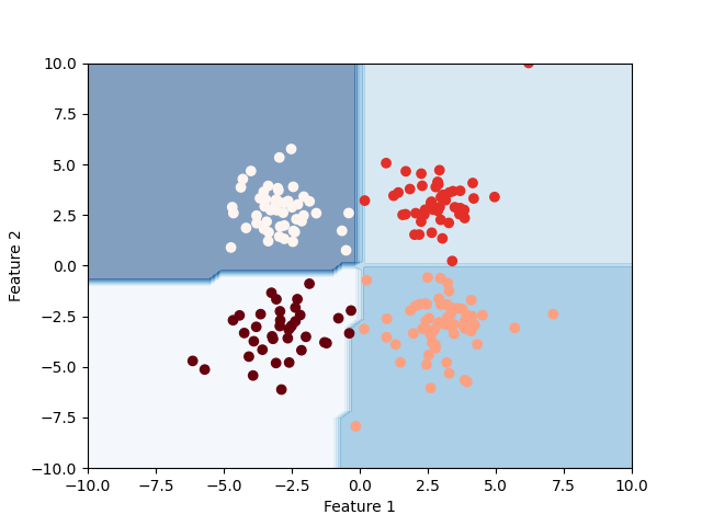
Example of decision boundary map for a mixture of Gaussian and low-degree Student distributions

This example is a retake from the experiment in the original GEMINI paper where we want to find the true clusters in a mixture of Gaussian that incorporates a low-degree-of-freedom student t-distribution. Consequently, this distribution generates sample that may seem like outliers if we are to expect only Gaussian distribution.

Unlike the paper, this example here is done with the gemclus.linear.LinearWasserstein instead of an MLP.

import numpy as np
from matplotlib import pyplot as plt

from gemclus.data import gstm
from gemclus.linear import LinearWasserstein

Generate the data

Taking 200 samples, 1 degree of freedom and not-so-far apart means

X, y = gstm(n=200, alpha=3, df=1, random_state=0)

Train the model for clustering

clf = LinearWasserstein(n_clusters=4, random_state=0, batch_size=50)
y_pred = clf.fit_predict(X)

Final Clustering

# Now, generate as well grid inputs to help drawing the decision boundary
x_vals = np.linspace(-10, 10, num=50)
y_vals = np.linspace(-10, 10, num=50)
xx, yy = np.meshgrid(x_vals, y_vals)
grid_inputs = np.c_[xx.ravel(), yy.ravel()]
zz = clf.predict(grid_inputs).reshape((50, 50))

# Plot decision boundary with predictions on top
plt.contourf(xx, yy, zz, alpha=0.5, cmap="Blues")
plt.scatter(X[:, 0], X[:, 1], c=y_pred, cmap="Reds_r")

plt.xlim(-10, 10)
plt.ylim(-10, 10)

plt.xlabel('Feature 1')
plt.ylabel('Feature 2')

plt.show()