Feature selection using the Sparse MMD OvA (MLP)

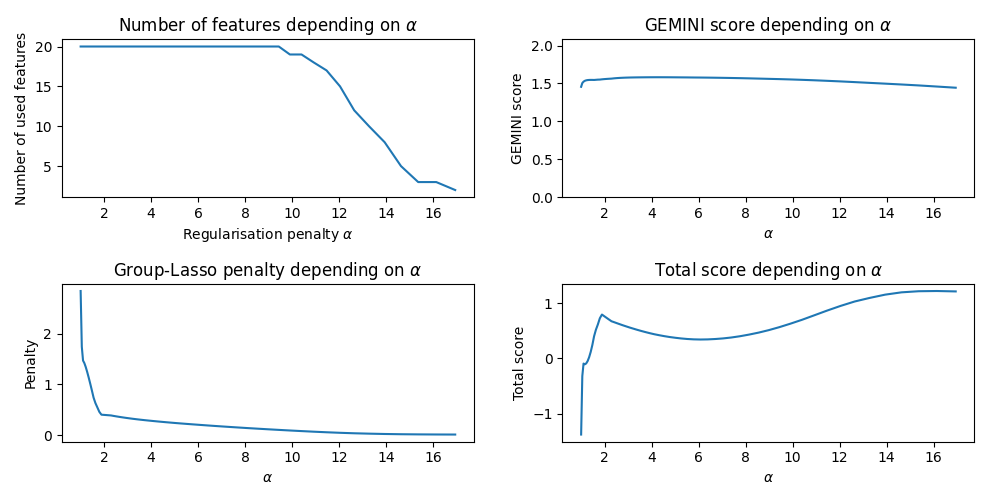
In this example, we ask the gemclus.sparse.SparseMLPMMD to perform a path where the regularisation penalty is progressively increased until all features but 2 are discarded. The model then keeps the best weights with the minimum number of features that maintains a GEMINI score close to 90% of the maximum GEMINI value encountered during the path.

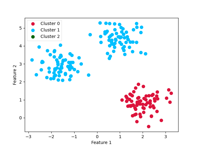
The dataset consists of 3 isotropic Gaussian distributions (so 3 clusters to find) in 2d with 48 noisy variables. Thus, the optimal solution should find that only 2 features are relevant and sufficient to get the correct clustering.

import numpy as np
from matplotlib import pyplot as plt
from sklearn import datasets

from gemclus.sparse import SparseMLPMMD

Load a simple synthetic dataset

# Generate samples on that are simple to separate
X, y = datasets.make_blobs(centers=3, cluster_std=0.5, n_samples=200, random_state=0)

# Add extra noisy variables
np.random.seed(0)
X = np.concatenate([X, np.random.normal(scale=0.5, size=(200, 18))], axis=1)

Train the model

Create the GEMINI clustering model (just a logistic regression) and call the .path method to iteratively select features through gradient descent.

clf = SparseMLPMMD(random_state=0, alpha=1, batch_size=50, max_iter=25, learning_rate=0.001)

# Perform a path search to eliminate all features
best_weights, geminis, penalties, alphas, n_features = clf.path(X)

Path results

Take a look at how our features are distributed

# Highlight the number of selected features and the GEMINI along decreasing increasing alphas
plt.figure(figsize=(10, 5))
plt.subplot(2, 2, 1)
plt.title("Number of features depending on $\\alpha$")
plt.plot(alphas, n_features)
plt.xlabel("Regularisation penalty $\\alpha$")
plt.ylabel("Number of used features")
plt.subplot(2, 2, 2)
plt.title("GEMINI score depending on $\\alpha$")
plt.plot(alphas, geminis)
plt.xlabel("$\\alpha$")
plt.ylabel("GEMINI score")
plt.ylim(0, max(geminis) + 0.5)
plt.subplot(2, 2, 3)
plt.title("Group-Lasso penalty depending on $\\alpha$")
plt.plot(alphas, penalties)
plt.xlabel("$\\alpha$")
plt.ylabel("Penalty")
plt.subplot(2, 2, 4)
plt.title("Total score depending on $\\alpha$")
plt.plot(alphas, np.array(geminis) - np.array(penalties) * alphas)
plt.xlabel("$\\alpha$")
plt.ylabel("Total score")
plt.tight_layout()
plt.show()

print(f"Selected features: {clf.get_selection()}")
print(f"The model score is {clf.score(X)}")
print(f"Top gemini score was {max(geminis)}, which settles an optimum of {0.9 * max(geminis)}")

Selected features: [0 1]
The model score is 1.4596486286280357
Top gemini score was 1.5824499242836227, which settles an optimum of 1.4242049318552605

Final Clustering

# Now, show the cluster predictions
y_pred = clf.predict(X)
X_0 = X[y_pred == 0]
X_1 = X[y_pred == 1]
X_2 = X[y_pred == 2]

ax0 = plt.scatter(X_0[:, 0], X_0[:, 1], c='crimson', s=50)
ax1 = plt.scatter(X_1[:, 0], X_1[:, 1], c='deepskyblue', s=50)
ax2 = plt.scatter(X_2[:, 0], X_2[:, 1], c='darkgreen', s=50)

leg = plt.legend([ax0, ax1, ax2],
                 ['Cluster 0', 'Cluster 1', 'Cluster 2'],
                 loc='upper left', fancybox=True, scatterpoints=1)
leg.get_frame().set_alpha(0.5)

plt.xlabel('Feature 1')
plt.ylabel('Feature 2')

plt.show()