Feature selection using the Sparse Linear MI (Logistic regression)

In this example, we ask the gemclus.sparse.SparseLinearMI to perform a path where the regularisation penalty is progressively increased until all features but 2 are discarded. The model then keeps the best weights with the minimum number of features that maintains a GEMINI score close to 50% of the maximum GEMINI value encountered during the path.

Contrary to the MMD sparse model, this one is not guided by specific kernel in the data space. That is why the acceptance threshold for best score is lowered to 50% instead of 90% like other models. A very similar model can be found in Discriminative Clustering and Feature Selection for Brain MRI Segmentation proposed by Kong et al. (2014).

The dataset consists of 3 isotropic Gaussian distributions (so 3 clusters to find) in 5d with 20 noisy variables. Thus, the optimal solution should find that only 5 features are relevant and sufficient to get the correct clustering.

import numpy as np
from matplotlib import pyplot as plt
from sklearn import metrics, decomposition

from gemclus.data import celeux_one
from gemclus.sparse import SparseLinearMI

Load a simple synthetic dataset

# Generate samples on that are simple to separate with additional p independent noisy variables
X, y = celeux_one(n=300, p=20, mu=1.7, random_state=0)

Train the model

Create the GEMINI clustering model (just a logistic regression) and call the .path method to iteratively select features through gradient descent.

clf = SparseLinearMI(random_state=0, alpha=1)

# Perform a path search to eliminate all features
best_weights, geminis, penalties, alphas, n_features = clf.path(X, keep_threshold=0.5)

# We expect the 5 first features
print(f"Selected features: {np.where(np.linalg.norm(best_weights[0], axis=1, ord=2) != 0)}")

Selected features: (array([ 0,  1,  2,  3,  4,  6, 11]),)

Final Clustering

# Now, evaluate the cluster predictions
y_pred = clf.predict(X)
print(f"ARI score is {metrics.adjusted_rand_score(y_pred, y)}")

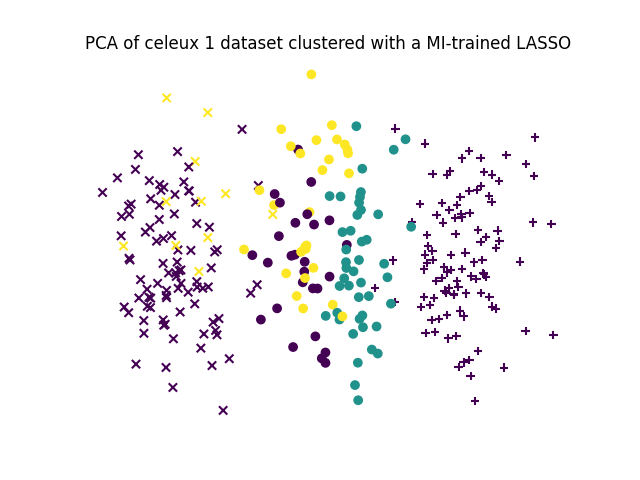
# Let's make a small PCA for visualisation purpose and distinguish true labels from clustering labels
X_pca = decomposition.PCA(n_components=2).fit_transform(X)

for k in range(3):
    class_indices, = np.where(y==k)
    plt.scatter(X_pca[class_indices,0], X_pca[class_indices,1], c=y_pred[class_indices], marker=["+","x","o"][k])
plt.axis("off")
plt.title("PCA of celeux 1 dataset clustered with a MI-trained LASSO")
plt.show()

ARI score is 0.458336976163333