Feature selection using the Sparse MMD OvO (Logistic regression)

In this example, we ask the gemclus.sparse.SparseLinearMMD to perform a path where the regularisation penalty is progressively increased until all features but 2 are discarded. The model then keeps the best weights with the minimum number of features that maintains a GEMINI score close to 90% of the maximum GEMINI value encountered during the path.

The dataset consists of 3 isotropic Gaussian distributions (so 3 clusters to find) in 5d with 20 noisy variables. Thus, the optimal solution should find that only 5 features are relevant and sufficient to get the correct clustering.

import numpy as np
from matplotlib import pyplot as plt
from sklearn import metrics

from gemclus.data import celeux_one
from gemclus.sparse import SparseLinearMMD

Load a simple synthetic dataset

# Generate samples on that are simple to separate with additional p independent noisy variables
X, y = celeux_one(n=300, p=20, mu=1.7, random_state=0)

Train the model

Create the GEMINI clustering model (just a logistic regression) and call the .path method to iteratively select features through gradient descent.

clf = SparseLinearMMD(random_state=0, alpha=1, ovo=True)

# Perform a path search to eliminate all features
best_weights, geminis, penalties, alphas, n_features = clf.path(X)

Path results

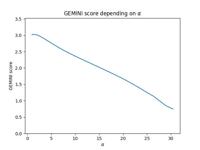
Take a look at how the GEMINI score decreased

print(f"The model score is {clf.score(X)}")
print(f"Top gemini score was {max(geminis)}, which settles an optimum of {0.9 * max(geminis)}")

# Highlight the number of selected features and the GEMINI along decreasing increasing alphas
plt.title("GEMINI score depending on $\\alpha$")
plt.plot(alphas, geminis)
plt.xlabel("$\\alpha$")
plt.ylabel("GEMINI score")
plt.ylim(0, max(geminis) + 0.5)
plt.show()

# We expect the 5 first features
print(f"Selected features: {np.where(np.linalg.norm(best_weights[0], axis=1, ord=2) != 0)}")

The model score is 2.8259728240495163
Top gemini score was 3.0249912491496707, which settles an optimum of 2.7224921242347038
Selected features: (array([0, 1, 2, 3, 4]),)

Final Clustering

# Now, evaluate the cluster predictions
y_pred = clf.predict(X)
print(f"ARI score is {metrics.adjusted_rand_score(y_pred, y)}")

ARI score is 0.83290627605772