Grouped Feature selection with a linear model

In this example, we ask the gemclus.sparse.SparseLinearMMD to perform a path where the regularisation penalty is progressively increased until all features but 2 are discarded. Moreover, we will produce some categorical variables that are one-hot-encoded and constrain the model to consider these features altogether using the groups option of the model.

The dataset consists of 2 binomial variables which parameters depend on the cluster (2 clusters to find) with 8 noisy variables. Thus, the optimal solution should find that only 2 features are relevant and sufficient to get the correct clustering.

import numpy as np
from matplotlib import pyplot as plt

from gemclus.sparse import SparseLinearMMD

np.random.seed(0)

Load a simple synthetic dataset

# Generate the informative variables that will be the outcome of multinomial distributions
X1_class_1 = np.random.multinomial(n=1, pvals=np.array([0.05, 0.45, 0.45, 0.05]), size=(50,))
X2_class_1 = np.random.multinomial(n=1, pvals=np.array([0.1, 0.1, 0.8]), size=(50,))
X_class_1 = np.concatenate([X1_class_1, X2_class_1], axis=1)
X1_class_2 = np.random.multinomial(n=1, pvals=np.array([0.45, 0.05, 0.05, 0.45]), size=(50,))
X2_class_2 = np.random.multinomial(n=1, pvals=np.array([0.8, 0.1, 0.1]), size=(50,))
X_class_2 = np.concatenate([X1_class_2, X2_class_2], axis=1)
X_informative = np.concatenate([X_class_1, X_class_2], axis=0) * 2

# Generate noisy variables
X_noise = np.random.normal(size=(100, 8))

X = np.concatenate([X_informative, X_noise], axis=1)

# The true cluster assignments
y = np.repeat(np.arange(2), 50)

# Finally, write out the partition of the dataset
groups = [np.arange(4), np.arange(4, 7)]
for i in range(8):
    groups += [np.array([i + 7])]

print(groups, X.shape)


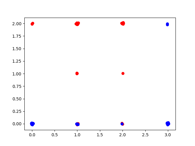
# Visualise clusters
def rand_jitter(data):
    return data + np.random.randn(len(data)) * 0.01


plt.scatter(rand_jitter(X1_class_1.argmax(1)), rand_jitter(X2_class_1.argmax(1)), c="red")
plt.scatter(rand_jitter(X1_class_2.argmax(1)), rand_jitter(X2_class_2.argmax(1)), c="blue")
plt.show()

[array([0, 1, 2, 3]), array([4, 5, 6]), array([7]), array([8]), array([9]), array([10]), array([11]), array([12]), array([13]), array([14])] (100, 15)

Train the model

Create the GEMINI clustering model (just a logistic regression) and call the .path method to iteratively select features through gradient descent.

clf = SparseLinearMMD(groups=groups, random_state=0, alpha=1)

# Perform a path search to eliminate all features, we lower the threshold to 80% of the max GEMINI in feature selection
best_weights, geminis, penalties, alphas, n_features = clf.path(X, keep_threshold=0.8)

Path results

Take a look at how our features are distributed

print(f"Selected features: {np.where(np.linalg.norm(best_weights[0], axis=1, ord=2) != 0)}")
print(f"The model score is {clf.score(X)}")
print(f"Top gemini score was {max(geminis)}, which settles an optimum of {0.9 * max(geminis)}")

Selected features: (array([0, 1, 2, 3, 4, 5, 6]),)
The model score is 1.3111799799449613
Top gemini score was 1.5884698387322584, which settles an optimum of 1.4296228548590326